Spiros Chavlis

🌟 Overall, we show that implementing dendritic properties can significantly enhance the learning capabilities of ANNs, boosting accuracy and efficiency. These findings hold great promise for optimizing the sustainability and effectiveness of ML algorithms! 🧠✨ #AI #MachineLearning #Dendrites (14/14)

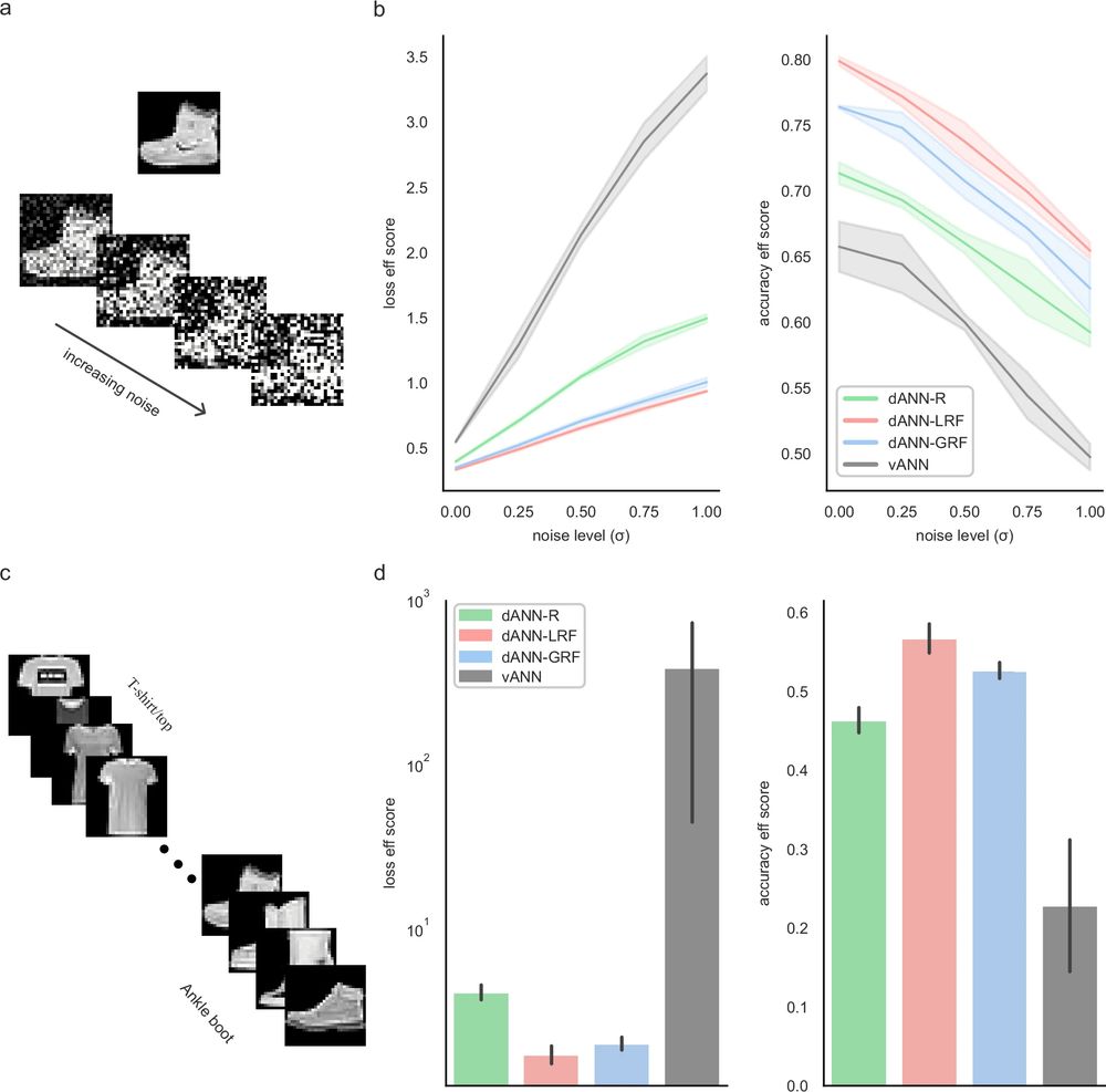
a An example of one FMNIST image with variable Gaussian noise. Sigma (σ) is the standard deviation of the Gaussian noise. b Testing loss (left) and accuracy (right) efficiency scores for all models and noise levels. Shades represent one standard deviation across N = 5 network initializations for each model. c The sequential learning task. d As in (b), but showing the loss (left) and accuracy (right) efficiency scores for the sequential task. Errorbars denote one standard deviation across N = 5 initializations for each model. See Table 2 and Supplementary Table 3 for the accuracy and loss values.

🔍 Finally, we crafted challenging scenarios for traditional ANNs, starting with added noise and sequentially feeding batches of the same class. Our findings show that dANNs with RFs exhibit greater robustness, accuracy, and efficiency, especially as task difficulty increases. (13/14)

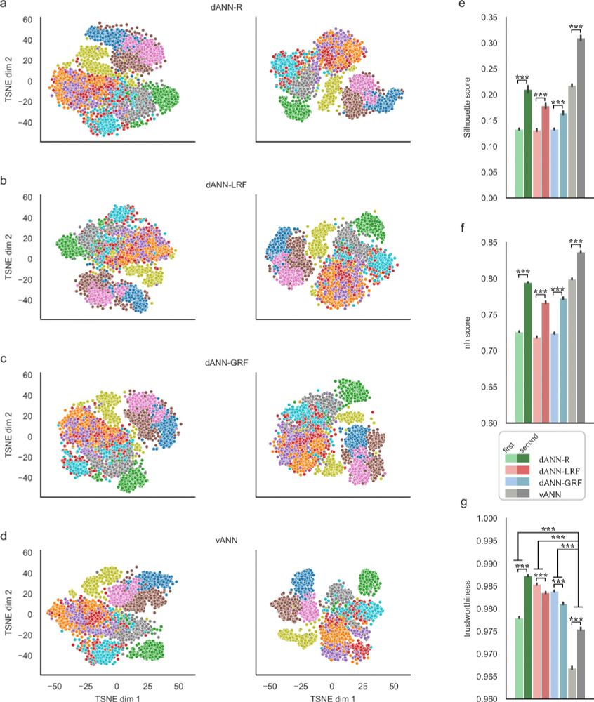
a–d TSNE projections of the activations for the first (left column) and the second (right column) hidden layers corresponding to the three dANN and the vANN models. Different colors denote the image categories of the FMNIST dataset. While the figure shows the results of one run, the representations are consistent across 10 runs of the TSNE algorithm (data not shown). e Silhouette scores of the representations. f Neighborhood scores of the representations, calculated using 11 neighbors. g Trustworthiness of the representations, calculated using 11 neighbors. In all barplots the error bars represent the 95% confidence interval across N = 5 initializations for each model and 10 runs of the TSNE algorithm per initialization. Stars denote significance with unpaired t-test (two-tailed) with Bonferroni’s correction.

🔍Rather than becoming class-specific early, dANNs show mixed-selectivity in both layers. This enhances trustworthy representations, achieving high accuracy with less overfitting and fewer, fully utilized params. (12/14)

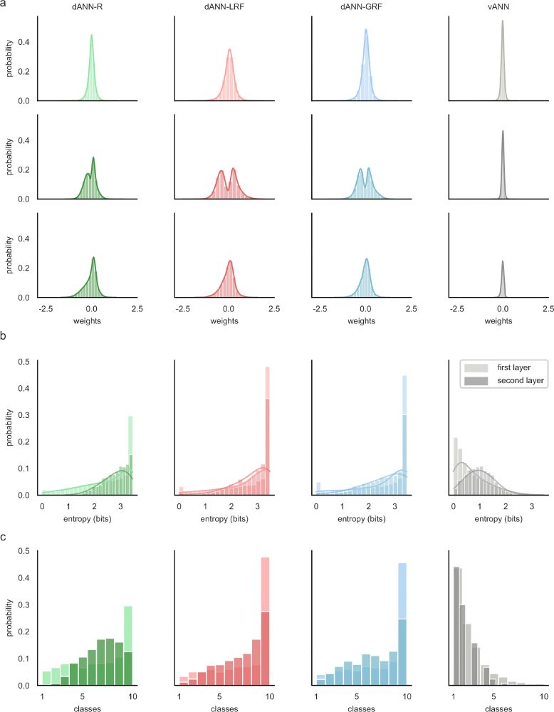
a Weight probability density functions after training for dANN-R, dANN-GRF, dANN-LRF, and vANN. The density functions are built by concatenating all weights across N = 5 initializations for each model. First hidden layer (top row), second hidden layer (middle row), and output layer (bottom row) weights are shown. Both x and y axes are shared across all subplots for visual comparison among the density plots. Supplementary Table 2 contains the kurtosis, skewness, and range of all KDE plots. b Probability density function of the entropy (bits) for the first (normal color) and second (shaded color) hidden layer, respectively. Entropies are calculated using the activations of each layer for all test images of FMNIST (see Methods). Silent nodes have been excluded from the visualization. Higher values signify mixed selectivity, whereas low values indicate class specificity. c Probability density functions of selectivity for both layers (different color shades) and all models (columns). For all histograms, the bins are equal to the number of classes, i.e., for the FMNIST dataset.

🔍 To understand dANN's edge over vANNs, we analyzed weight distributions after training on Fashion MNIST. ANNs fully utilize their parameters, especially dendrosomatic weights. Entropy and selectivity distributions also indicate different strategies for tackling the same classification task. (11/14)

The following models were compared: dANN-R and vANN-R with random input sampling (light and dark green), dANN-LRF and vANN-LRF with local receptive field sampling (light and dark red), dANN-GRF and vANN-GRF with global receptive field sampling (light and dark blue), and pdANN and vANN with all-to-all sampling (light and dark purple). a Number of trainable parameters that each model needs to match the highest test accuracy of the respective vANN. b The same as in a, but showing the number of trainable parameters required to match the minimum test loss of the vANN. c Difference (Δ) in accuracy efficiency score between the structured (dANN/pdANN) and vANN models. Test accuracy is normalized with the logarithm of trainable parameters times the number of epochs needed to achieve minimum validation loss. The score is bounded in [0, 1]. d Same as in c, but showing the difference (Δ) of the loss efficiency score. Again, we normalized the test score with the logarithm of the trainable parameters times the number of epochs needed to achieve minimum validation loss. The score is bounded in [0, ∞). In all barplots the error bars represent one standard deviation across N = 5 initializations for each model.

🔍 Our findings highlight that structured connectivity and restricted input sampling in dANNs yield significant efficiency gains in image classification over classical vANNs! When comparing dANNs and pdANN to vANN, we found that RFs boost efficiency, but not to the extent of dANNs. (10/14)

The comparison is made between the three dendritic models, dANN-R (green), dANN-LRF (red), dANN-GRF (blue), the partly-dendritic model pdANN (purple) and the vANN (grey). a Number of trainable parameters that each model needs to match the highest test accuracy of the vANN. b The same as in a, but showing the number of trainable parameters required to match the minimum test loss of the vANN. c Accuracy efficiency scores of all models across the five datasets tested. This score reports the best test accuracy achieved by a model, normalized with the logarithm of the product of trainable parameters with the number of epochs needed to achieve minimum validation loss. The score is bounded in [0, 1]. d Same as in c, but showing the loss efficiency score. Here the minimum loss achieved by a model is normalized with the logarithm of the trainable parameters times the number of epochs needed to achieve minimum validation loss. The score is bounded in [0, ∞). In all barplots the error bars represent one standard deviation across N = 5 initializations for each model.

📈 To validate the benefits of dendritic features, we tested dANN models on five benchmark datasets. Results showed that top dANN models matched or even outperformed the best vANNs in accuracy and loss! Additionally, dANNs proved significantly more efficient across all datasets. (9/14)

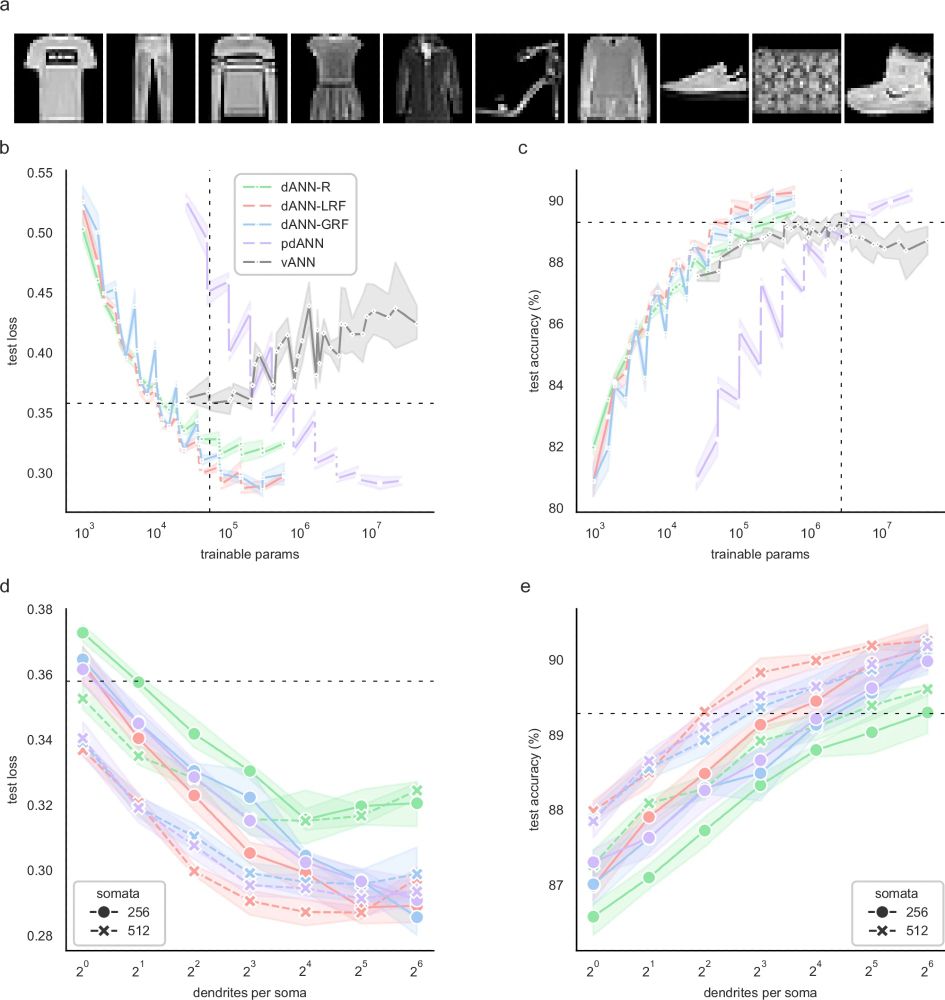
a The Fashion MNIST dataset consists of 28×28 grayscale images of 10 categories. b Average test loss as a function of the trainable parameters of the five models used: A dendritic ANN with random inputs (dANN-R, green), a dANN with LRFs (red), a dANN with GRFs (blue), a partly-dendritic ANN with all-to-all inputs (pdANN, purple), and the vANN with all-to-all inputs (grey). Horizontal and vertical dashed lines denote the minimum test loss of the vANN and its trainable parameters, respectively. The x-axis is shown in a logarithmic scale (log10). c Similar to B, but depicting the test accuracy instead of the loss. d Test loss as a function of the number of dendrites per somatic node for the three dANNs and the pdANN model. The linestyle (solid and dashed) represents different somatic numbers. The dashed horizontal line represents the minimum test loss of the vANN (512-256 size of its hidden layers, respectively). The x-axis is shown in a logarithmic scale (log2). e Similar to (d), but showing the test accuracy instead of the loss. The dashed horizontal line represents the maximum test accuracy of the vANN (2048-512 size of its hidden layers, respectively). Note that while all models have the same internal connectivity structure, the pdANN model (purple) has a much larger number of trainable parameters due to its all-to-all input sampling. For all panels, shades represent the 95% confidence interval across N = 5 initializations for each model.

Our dANN and pdANN models show improved learning with network sizes, lower loss, and better accuracy! More importantly, they maintain performance and stability as the number of layers increases. This reveals their potential for deeper architectures! 🧠💪 (8/14)

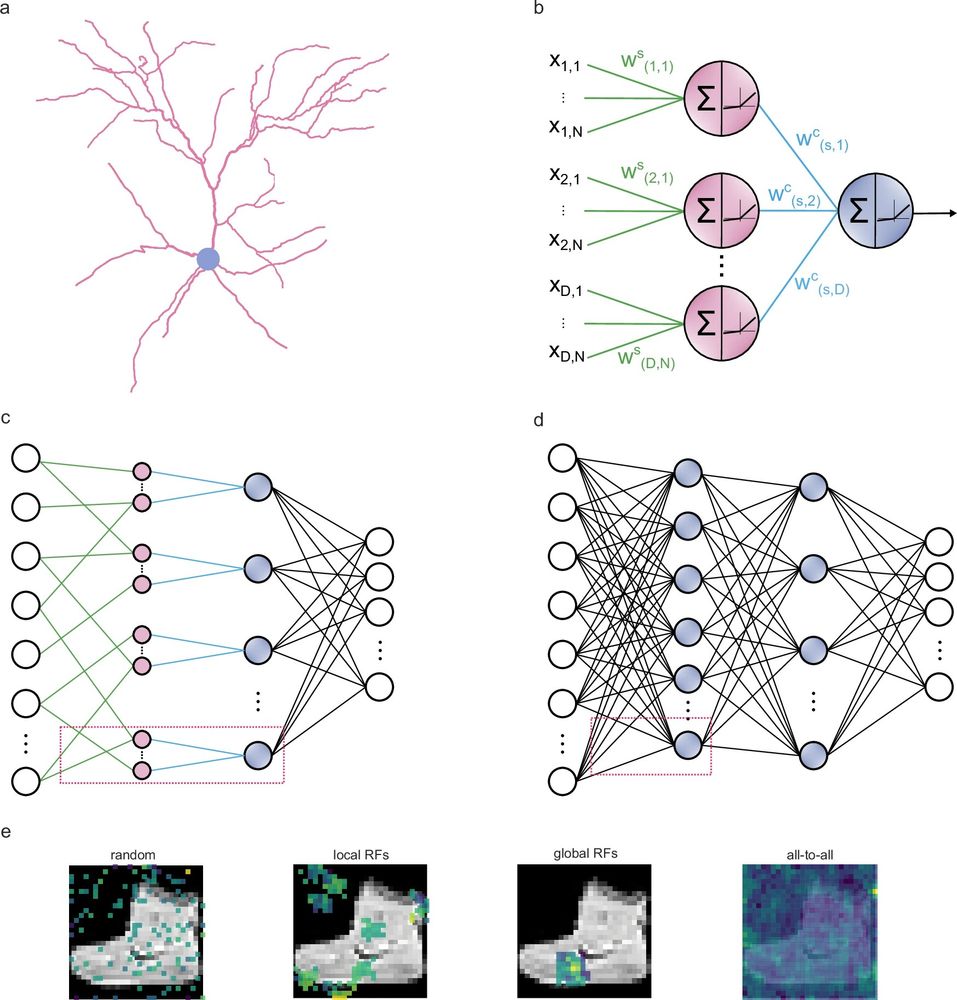
a Example of a layer 2/3 pyramidal cell of the mouse primary visual cortex (dendrites: pink; soma: grey) that served as inspiration for the artificial dendritic neuron in b. The morphology was adopted from Park et al. (ref 127). b The dendritic neuron model consists of a somatic node (blue) connected to several dendritic nodes (pink). All nodes have a nonlinear activation function. Each dendrite is connected to the soma with a (cable) weight, w(d,s)^c, where d and s denote the dendrite and soma indices, respectively. Inputs are connected to dendrites with (synaptic) weights, w(d,n)^s, where d and n are indices of the dendrites and input nodes, respectively. dϵ{1, D}, nϵ{1, N}, N denotes the number of synapses each dendrite receives, and D the number of dendrites per soma s. c The dendritic ANN architecture. The input is fed to the dendritic layer (pink nodes), passes a nonlinearity, and then reaches the soma (blue nodes), passing through another nonlinearity. Dendrites are connected solely to a single soma, creating a sparsely connected network. d Typical fully connected ANN with two hidden layers. Nodes are point neurons (blue) consisting only of a soma. e Illustration of the different strategies used to sample the input space: random sampling (R), local receptive fields (LRF), global receptive fields (GRF), and fully connected (F) sampling of input features. Examples correspond to the synaptic weights of all nodes that are connected to the first unit in the second layer. The colormap denotes the magnitude of each weight. The image used in the background is from the Fashion MNIST (FMNIST) dataset.

🔍 We explored three input sampling methods for dendritic ANN models (dANN): a) random (R), b) local receptive fields (LRF), and c) global receptive fields (GRF). We also included a fully connected sampling (F), calling it a partly-dendritic ANN (pdANN) 🧠✨. (7/14)

🌱 Our proposed architecture features partially sampled inputs fed into a structured dendritic layer, which connects sparsely to the somatic layer! 🧠✨

Inspired by the receptive fields of visual cortex neurons, this approach mimics the locally connected networks. (6/14)

Might a Single Neuron Solve Interesting Machine Learning Problems Through Successive Computations on Its Dendritic Tree? Physiological experiments have highlighted how the dendrites of biological neurons can nonlinearly process distributed synaptic inputs. However, it is unclear how aspects of a dendritic tree, such as ...

Inspired by the work of @ilennaj.bsky.social and @kordinglab.bsky.social, doi.org/10.1162/neco..., we propose a bio-inspired dendritic architecture to enhance learning in ANNs using backpropagation! (5/14)

🌿 Dendrites generate local regenerative events and mimic the spiking profile of a soma, acting like multi-layer ANNs! 🤯 doi.org/10.1016/s089...

Dends enable complex computations, like logical operations, signal amplification, and more 🧠💡
doi.org/10.1016/j.co...
www.nature.com/articles/s41... (4/14)

🧠 The biological brain processes, stores, and retrieves vast info quickly and efficiently, using minimal energy! ⚡️ Meanwhile, ML/AI systems are energy-hungry! 🤖💡 Our solution? Dendrites! 🌱✨(3/14)

Dendrites endow artificial neural networks with accurate, robust and parameter-efficient learning - Nature Communications Artificial neural networks, central to deep learning, are powerful but energy-consuming and prone to overfitting. The authors propose a network design inspired by biological dendrites, which offe...

Before we dive deeper into it, I would like to thank my amazing supervisor, @yiotapoirazi.bsky.social, for all her support and kindness during my 12 years in the @dendritesgr.bsky.social. The paper can be found @naturecomms.bsky.social www.nature.com/articles/s41... (2/14)

🚀 Excited to share my latest paper! 📄✨ This project started at the beginning of the pandemic and took longer than expected, but that’s the beauty of science! 🧬🔬 Check it out in the following threads! #PandemicProjects

My post comes a bit late because of TAing duties in @imbizo.bsky.social🇿🇦(1/14)