RPubs - Reproducible data analysis using tidyverse R
Updated my “Reproducible data analysis using tidyverse R” slides in preparation for a workshop at UVA tomorrow: rpubs.com/bpbond/1392825 #rstats
03.02.2026 14:17 — 👍 8 🔁 4 💬 0 📌 0
Yes, the VOD will be available (I think at the same link) shortly after the end of the livestream and it will remain available indefinitely
03.02.2026 20:06 — 👍 2 🔁 0 💬 0 📌 0
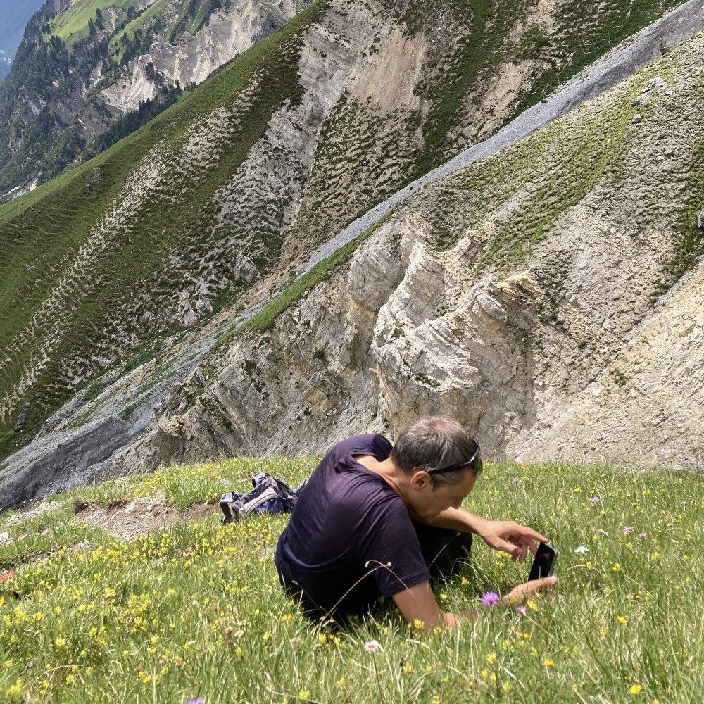
LOL, it’s meant to be me (the geographer) looking up to the scientists at the pinnacle of academia.
It’s from an insult the Lindzen, a noted climate, denialist made against the IPCC (as being composed of people from the bottom of the heap, like geographers)
I have two degrees in geography
03.02.2026 17:10 — 👍 3 🔁 0 💬 0 📌 0
Basically, they’re just GAMs but with penalised splines applied at different scales of data, average of all data, group specific smooths, subject specific random smooths etc, but the paper goes into the detail c. 2018-2019
03.02.2026 14:32 — 👍 1 🔁 0 💬 0 📌 0

gavinsimpson gratia Q A · Discussions
Explore the GitHub Discussions forum for gavinsimpson gratia in the Q A category.
There’ll be a live Q&A—post questions in advance via the gratia GitHub Discussions (tag livestream), and upvote the ones you want answered.
Post your questions: github.com/gavinsimpson...
03.02.2026 12:57 — 👍 3 🔁 0 💬 0 📌 0
During the livestream, I'll be covering:
• what GAMs are and how they work
• recent mgcv updates (incl. Hierarchical GAMs)
• new features in gratia
• deeper inference with marginaleffects
03.02.2026 12:57 — 👍 7 🔁 0 💬 2 📌 0

What's new in the world of Generalized Additive Models
YouTube video by Bottom of the Heap
🚨 GAMs have moved on—so it’s time for an update.
On March 3, 2026 (17:00–19:00 CET) I’ll be livestreaming an updated introduction to Generalized Additive Models in R
📺 YouTube livestream link: youtube.com/live/A9U8e1K...
#RStats #mgcv #GAMs #gratia #statistics 🧪
03.02.2026 12:57 — 👍 82 🔁 36 💬 4 📌 0
All my #rstats ebooks are now in the quarto format, and hosted on Quarto Pub. Their old bookdown links will all be dead by the weekend.
1/3
28.01.2026 15:34 — 👍 87 🔁 24 💬 5 📌 1

European leaders warn of ‘downward spiral’ after Trump threatens tariffs over Greenland – Europe live
Denmark, Norway, Sweden, the UK, France, Germany, the Netherlands and Finland will face tariffs from 1 February
Isn’t it about time that European countries tax the shit out of the massive US tech firms looting them (they exploit every loophole to pay relatively little tax)?
If he raises tariffs, we raise taxes on their revenue.
www.theguardian.com/world/live/2...
17.01.2026 20:04 — 👍 2 🔁 0 💬 0 📌 0
While Ukrainians face 30+ hour blackouts, Moscow's Higher School of Economics hosts seminars with top international speakers-then uses the same rooms for drone fundraisers. Academics don't get paid for seminars. So why present at an institution actively funding mass murder of Ukrainians? #Econsky
15.01.2026 15:20 — 👍 21 🔁 4 💬 1 📌 0
If this is a general “penalties = priors” thing I don’t think that is generally true. There are specific cases where they work out to be equivalent to a particular (possibly improper) prior. This is what underlies mgcv and IIRC also INLA (but I’m less familiar with the latter)
15.01.2026 07:46 — 👍 0 🔁 0 💬 0 📌 0
I think that would be using an “old style” or “scheffer style” random effect interpretation sensu Hodges. We don’t tend to think our spline is a draw from a multivariate Gaussian as if it were some weird set of random effects but we use this as a computational convenience, AKA “new style” ranefs
15.01.2026 07:40 — 👍 0 🔁 0 💬 0 📌 0
Isn’t this called maximum a posteriori estimation? What mgcv does is an empirical Bayesian edtimate. The “penalty” is an improper Gaussian prior on the smooth coefs and lambda is inversely proportional to a variance parameter. I’m away from my books & other stuff but I think this is in Wood 2011
15.01.2026 07:35 — 👍 1 🔁 0 💬 0 📌 0
📈 Registrations now open!
Time Series Analysis & Forecasting in R
🗓 20–24 July| 🌍 Online
A very hands-on course on dynamic GLMs/GAMs for ecological time series using {mvgam} & {brms}. Bayesian models, nonlinear effects, forecasting & live coding in R.
www.physalia-courses.org/courses-work...
07.01.2026 09:19 — 👍 5 🔁 5 💬 1 📌 0
Ok science hivemind 🧪. I have a distinct memory of an awesome graphic in a paper about how environmental filtering and biotic interactions determine whether an organism can live in any given place. Almost like multiple filter layers on top of another. Does anyone have a preferred graphic of this?
07.01.2026 11:56 — 👍 2 🔁 3 💬 2 📌 0
Interested in Species Distribution Modeling (SDM) and Ecological Niche Modeling (ENM) in R? Don’t miss this chance to level up your skills! The course is nearly full — www.physalia-courses.org/courses-work...
#SDM #ENM #RStats #Ecology #DataScience
06.01.2026 08:30 — 👍 4 🔁 2 💬 1 📌 1
If you mentor scientific writers, teach a course with written assignments, or anything similar, you know how much work is involved, and how difficult it can be to provide the guidance developing writers need. This book is for you!
2/2
05.01.2026 11:57 — 👍 6 🔁 2 💬 2 📌 0

Teaching and Mentoring Writers in the Sciences: An Evidence-Based Approach
Scientific writing is hard (but my book can help) – but teaching scientific writing is even harder. Nearly all of us teach writing – sometimes in a formal classroom setting, sometimes as advisors t…
Over the holiday, while folks were on well-deserved breaks, our new book was released!
Mentoring writers is hard - we can make it easier for you. Please help spread the word - repost this, tell your colleagues, etc.
scientistseessquirre...
1/2
05.01.2026 11:57 — 👍 59 🔁 21 💬 3 📌 2

course schedule as a table. Available at the link in the post.
I'm teaching Statistical Rethinking again starting Jan 2026. This time with live lectures, divided into Beginner and Experienced sections. Will be a lot more work for me, but I hope much better for students.
I will record lectures & all will be found at this link: github.com/rmcelreath/s...
09.12.2025 13:58 — 👍 658 🔁 236 💬 12 📌 20

We are recruiting several PhD students. If you are interested in conservation conflicts, population ecology, quantitative ecology, or biodiversity, check these projects out (links in the thread, feel free to reach out):
28.12.2025 23:35 — 👍 46 🔁 50 💬 2 📌 3
Congratulations Stephen 🎉🍾
31.12.2025 13:22 — 👍 1 🔁 0 💬 1 📌 0
Here is a little piece about the day of my final Monkey Cage recording - a couple of weeks ago in beautiful #manchester www.bigissue.com/opinion/robi...
26.12.2025 17:07 — 👍 260 🔁 39 💬 6 📌 1
Goodbye, Monkey Cage - not as infinite as I imagined
25.12.2025 11:55 — 👍 986 🔁 101 💬 97 📌 16

Photo showing a freshly baked rich fruit cake that is my mum’s family Christmas cake recipe
Probably should have been made a month or more ago, but better late than never. Made my mum’s family Christmas cake recipe for the first time since moving to 🇩🇰
23.12.2025 22:27 — 👍 10 🔁 0 💬 0 📌 0

A mystery seed from a Breckland, eastern England ghostpingo core as found by @hayleymcmechan.bsky.social. help oh botanists!!! 1 mm scale @annasolcova.bsky.social @jo-the-botanist.bsky.social @bramblebotanist.bsky.social @timholtwilson.bsky.social
21.12.2025 19:07 — 👍 20 🔁 5 💬 7 📌 0
The first global conference on how data visualisation can support understanding and decision-making on climate change.
𝗕𝗼𝗹𝗼𝗴𝗻𝗮, 𝗜𝘁𝗮𝗹𝘆
4–6 November 2026
#datavis #climate
ℹ️ visualisingclimate.com
Join the UseR! at Warsaw!
We’re excited to announce that UseR! Conference in 2026 is being hosted in Warsaw, bringing together data scientists, statisticians, and researchers from across the world.
7-9 July, 2026
https://user2026.r-project.org/
Scientist interested on how to achieve sustainable development.
B.Sc. double-majored in physics & applied math. Aspiring interdisciplinary mathematician. Data driven, information-theoretic, Bayesian approaches to modeling complex & nonequilibrium systems.
They/Them
Most likes are papers added to my literature search
statistics Associate Prof in UCD 🇮🇪 working on problems in genetics, social networks, etc. 🏃🏻➡️🚲
maths.ucd.ie/~mst
Ornithologist and biogeographer. Working on the global macroecology of bird-window collisions and on the genetics of faunal adaptation to mangroves. Obsessed with pittas. Previously at the University of New Mexico, now a postdoc at iDiv in Leipzig.
Data Science is my thing. Fan of FOSS. A good day is writing code in R (#rstats) with no meetings and nary a Microsoft product in sight. Introvert, appreciator of excellence. Should update avatar to have a gray beard now...
@embiggendata@c.im on Mastodon
Macroecologist | species distribution dynamics and biodiversity change | from post-glacial migration to recent global change and biological invasions | wsl.ch/en/
❤️📊 | 🗣️DE|EN|FR | #rstats | #econsky
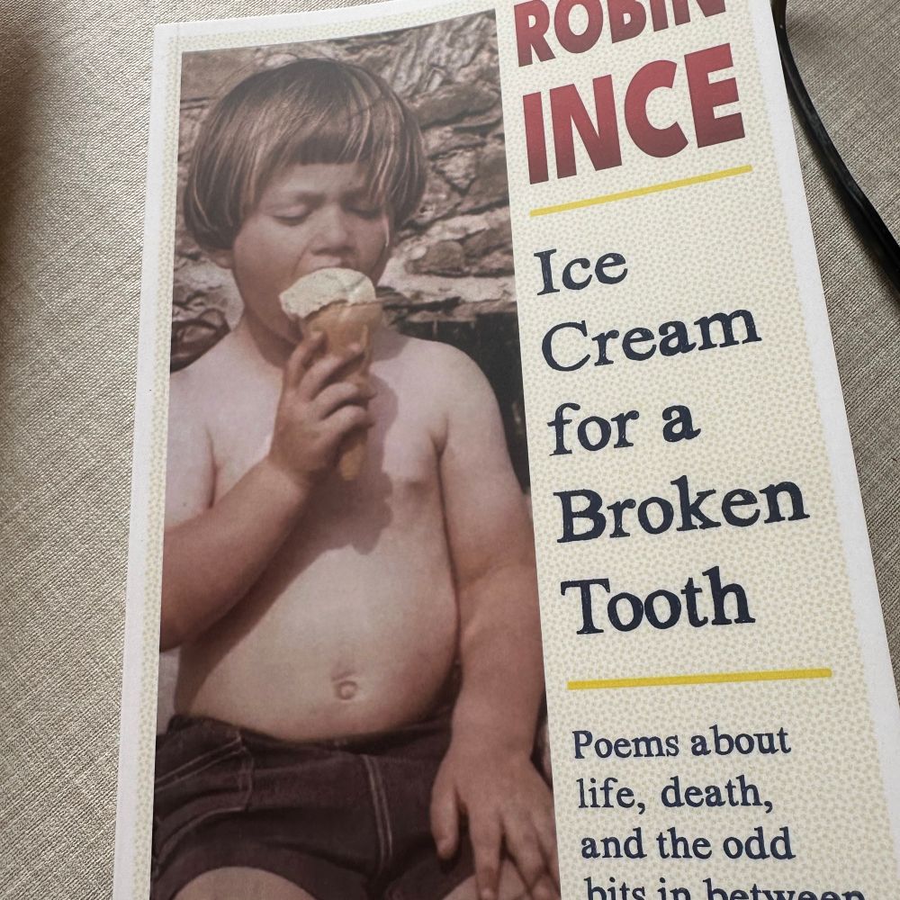
Two books published this year - Normally Weird & Weirdly Normal and poetry collection Ice Cream for a Broken Tooth
Glaswegian Londoner, Statistician, Immunologist, Virologist, Data Scientist, Celtic Fan.
Researcher in chemical ecology of plant-insect interactions @cefemontpellier @cnrs
PhD | Marine Ecologist | Postdoctoral Fellow @mncn-bgcg.bsky.social | Effects of Climate Change on Biodiversity | he/ him | Dad
Senior Scientist and Bioinformatician at the New Zealand Institute for Bioeconomy Science | Helping improve agriculture in Aotearoa New Zealand
respect sampling variability
Data Scientist, #rstats
Might also post pictures of my weirder cat, I guess.
aquatic ecology, ecological modelling, biostatistics
Plant ecologist at Czech Academy of Sciences / Inst of Botany / Dept of Geoecology
forests, microclimate, biogeography