Surface Ocean CO₂ Atlas

Fig. 4: Simulated change signal of ocean–atmosphere CO₂ flux during the twentieth century (1991–2010 of hist minus ctrl), shown for the coastal ocean.

Moritz Mathis et al.* explore the mechanisms behind enhanced coastal CO₂ uptake.

doi.org/10.1038/s415...

#ocean #co2 #coast

*Fabrice Lacroix, Stefan Hagemann, David Marcolino Nielsen, Tatiana Ilyina & Corinna Schrum

Excited to announce that we will be hosting the 6th International Symposium on Oceans in a High CO2 World October 12 to 16th in Wellington at the Tākina event center! This conference will bring together marine climate change scientists from multiple disciplines. Save the date!

Yujun Liu, Yijun He and Yating Shao explore the impact of cold season Arctic cyclones on the carbon sink of the marginal sea ice zone.

doi.org/10.1016/j.sc...

#arctic #co2 #cyclone

Figure 1: Air–sea CO2 flux map of climatological annual mean (a–c) and 2015 interannual anomaly (d–f) between data products and MOM6-COBALT. A positive flux denotes an outgassing from the ocean to atmosphere. In panel (a), AS, BoB, SEIO denote Arabian Sea, Bay of Bengal, and southeastern Indian Ocean respectively. Sumatra, Java, SS, LS, and TS represent Sumatra island, Java island, Lombok Strait, Sunda Strait, and Timor Sea respectively. Arrows in panel (c and d) depict the ocean circulation of climatological annual mean and interannual anomaly for 2015, derived from MOM6-COBALT. Data products are from MPI SOM-FFN and OS-ETHZ-GRaCER. The interannual anomaly is averaged between August 2015 and July 2016.

Enhui Liao, Wenfang Lu, Liang Xue, and Yan Du attribute an anomalous drop in Indian Ocean CO₂ uptake to large-scale warming and reduced physical transport.

doi.org/10.1002/lol2...

#IndianOcean #carbon #co2

Figure 3: (a) The mean air-sea CO₂ flux density and (b) trend in the CO₂ flux density 1958–2019 in the historical simulation (simulation A) (c–f) The effects of the rising atmospheric CO₂ concentration and climate change on the trend in the CO₂ flux density obtained as the difference between two simulations with and without interannual variability and trends in the respective variable(s): (c) Atmospheric CO₂ concentration, (d) full climate variability and trends, (e) winds and (f) global warming. Positive values denote a trend toward more oceanic outgassing or less oceanic uptake, respectively. Hatched areas in (b–f) indicate a low significance of the trend (p-value > 0.05 applying a two-sided Wald Test with t-distribution).

Frauke Bunsen, Cara Nissen and Judith Hauck assess the impacts of climate change on the global ocean carbon sink

doi.org/10.1029/2023...

#ocean #carbon

Figure 4: Breakdown of uncertainty sources, compared seasonally. (a) July uncertainty sources (averaged 1990–2022) color indicating dominating source of uncertainty (k, pCO2, and wind). (b) Percentage each source contributes to total uncertainty, averaged latitudinally. (c, d) Same as (a, b) but for January.

Annika Jersild and Peter Landschützer show how the sources of uncertainty and bias in a neural network based air-sea CO₂ reconstruction vary in different ocean regions.

doi.org/10.1029/2023...

#ocean #flux #uncertainty

Figure 1: Map of the Eastern Mediterranean Sea with location of Heraklion Coastal Buoy (HCB), E1-M3A buoy and FINOKALIA atmospheric station (bottom left inset). Color tracks (z axis) indicated difference between observed and estimated sea surface pCO₂ (Δobs-est), using Equation 8 with in-situ temperature and pCO₂ measurements (from SOCAT dataset). Top right inset shows frequency of observations vs Δobs-est. In-situ data excluded values above latitude 39.8°N and data from the present study.

C. Frangoulis et al.* present two years of high-frequency carbonate system observations from the eastern Mediterranean.

doi.org/10.3389/fmar...

#ocean #mediterranean #carbon

Stamataki, Pettas, Michelinakis, King, Giannoudi, Tsiaras, Christodoulaki, Seppälä, Thyssen, Borges, Krasakopoulou

Figure 5: Annual mean CO₂ flux calculated from the SOCAT database. Flux is calculated using the SeaFlux method using the mean of three wind speed reanalysis products. Warm and cool colors indicate regions of carbon efflux and uptake, respectively. The near-global mean flux is −1.79 Pg C yr⁻¹.

Amanda Fay et al.* present new climatologies of mean ΔfCO and net sea–air CO flux for the global ocean.

doi.org/10.5194/essd...

#ocean #co2 #flux

*David Munro, Galen McKinley, Denis Pierrot, Stewart Sutherland, Colm Sweeney, Rik Wanninkhof

Global Analysis of Surface Ocean CO2 Fugacity and Air‐Sea Fluxes With Low Latency We demonstrate the capacity of statistical models to generate global maps of fCO2 and air-sea flux with a latency reduced to one month A decrease in the CO2 source for January to August 2023 diag...

Thi-Tuyet-Trang Chau, Frédéric Chevallier and Marion Gehlen use a set of biological, chemical, and physical predictors to produce global monthly maps of fCO₂ and air-sea CO₂ fluxes beyond the available SOCAT observations.

doi.org/10.1029/2023...

#ocean #co2 #flux

Unexpected decline in the ocean carbon sink under record-high sea surface temperatures in 2023 - Nature Climate Change The ocean carbon sink strengthened in previous warm El Niño years due to reduced CO2 outgassing in the tropics. Here the authors show that the ocean carbon sink declined in 2023 despite record-high se...

🌊 In 2023, the ocean carbon sink weakened for the first time in a record-hot year 🌡️🌎
Our new study in Nature Climate Change quantifies this unexpected decline and explains how it came about. 👇
doi.org/10.1038/s415...

Fig. 9: Statistical summary showing the mean pCO2 difference from the IC-Reference for each of the six measurement intervals defined in Fig. 4, ordered by instrument per group. The horizontal dashed lines divide the instruments' groups while the vertical gray dashed lines denote the 2, 5, and 10 μatm limits.

Tobias Steinhoff and 40+ co-authors present the results from a two-week intercomparison of 27 pCO₂ instruments (16 models)

doi.org/10.1002/lom3...

#ocean #co2

A Synthesis of Global Coastal Ocean Greenhouse Gas Fluxes We synthesize air-sea fluxes of CO2, nitrous oxide and methane in the global coastal ocean using observation-based products and ocean models The coastal ocean CO2 sink is 60% larger in ocean mode...

Laure Resplandy et al. (too many to fit here) present a global synthesis of coastal fluxes of carbon dioxide, nitrous oxide and methane across the globe.

doi.org/10.1029/2023...

#ocean #carbon #flux #coast

Some SOCAT services are currently offline due to ongoing IT issues with some servers. The outage is expected to last several days.

Main data downloads are unaffected.

Figure 2: Air-sea CO2 flux variance explained by the mesoscale. (a) CO2 flux variance associated with small scales (<nominal 2°); (b) Percentage of CO2 flux variance explained by small scales. Gray contours are mean sea surface height contours (CI = 20 cm) in the model.

Yiming Guo and Mary-Louise Timmermans examine the role of mesoscale processes on global air-sea CO₂ fluxes.

doi.org/10.1029/2024...

#ocean #co2

Figure 7: (a) Division of the coastal ocean into five coastal systems that present different key controls on the coastal CO2 dynamics in the mixed layer depth (MLD). For each of these five categories is associated a sketch (b–f) that presents the main control on the annual average CO2 sources/sinks and the variability on the seasonal timescale (red stars) in the MLD. Flux into the MLD increases CResponse.

Alizée Roobaert et al* discover the factors constraining the coastal air-sea CO₂ flux across the globe.

doi.org/10.1029/2023...

#ocean #co2 #flux #coast

Laure Resplandy, Goulven G. Laruelle, Enhui Liao, Pierre Regnier

Figure 1: CMEMS-LSCE-FFNN pCO₂ over the global ocean at a spatial resolution of 0.25∘. Temporal means of the model best estimate and 1σ uncertainty per grid cell over 1985–2021.

Thi-Tuyet-Trang Chau et al.* present CMEMS-LSCE, a 0.25° monthly reconstruction of the surface ocean carbonate system.

doi.org/10.5194/essd...

#ocean #co2

*Marion Gehlen, Nicolas Metzl, Frédéric Chevallier

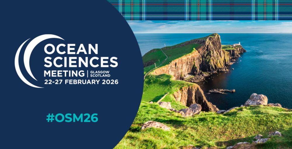
Ocean Sciences Meeting 2026 Join AGU, TOS, and ASLO for the Ocean Sciences Meeting, held 22-27 February 2026, in Glasgow, Scotland. The meeting is the flagship conference for the ocean sciences community and the larger ocean-con...

🔊We are pleased to announce our SOCOM session

'SOLAS and SOCOM: Understanding interactions and feedbacks between the ocean and atmosphere'

was accepted for #OSM26 in Feb 2026.
Co-chaired by Dr Thea Heimdal and Dr Amanda Fay.

www.agu.org/Ocean-Scienc...

#OC4C @lamont.columbia.edu

Judith Hauck and 13 others come together to review the Southern Ocean carbon cycle over 20+ years.

doi.org/10.1029/2023...

#SouthernOcean #carbon

Fig. 1: Diapycnal mixing in the Southern Ocean State Estimate (SOSE). The distribution of diapycnal mixing in the Southern Ocean, constructed as the sum of contributions from tides and topographically generated lee waves. This mixing is shown averaged in depth over the top/bottom 2 km in panel A/B, and zonally over the Southern Ocean in (c). These maps are used in the spatially variable mixing map experiment (ExVar). For reference, a zonally averaged map of the storm-induced mixing, as parameterized through GGL90 parameterization in B-SOSE, is also shown in panel (d). The pink lines on (a) and (b) show the annual mean extent of sea ice. Note that the range of the color bar in panel (d) is different from the other panels.

Elizabeth Ellison, Ali Mashayek and Matthew Mazloff investigate how diapycnal mixing variability can affect air-sea CO₂ fluxes in the Southern Ocean.

doi.org/10.1029/2023...

#SouthernOcean #co2 #flux

Estimating marine carbon uptake in the northeast Pacific using a neural network approach Abstract. The global ocean takes up nearly a quarter of anthropogenic CO2 emissions annually, but the variability in this uptake at regional scales remains poorly understood. Here we use a neural netw...

Patrick Duke et al.* estimate the regional marine CO₂ fluxes in the northeast Pacific

doi.org/10.5194/bg-2...

#ocean #pacific #carbon #co2

*Roberta Hamme, Debby Ianson, Peter Landschützer, Mohamed Ahmed, Neil Swart, Paul Covert

New session confirmed for Ocean Science 2026 in Glasgow: The Southern Ocean Carbon Sink: processes, observations, and change. agu.confex.com/agu/osm26/pr...

#OSM26 #SouthernOcean #carbon

Fig 1: Central panel showing biomes used for this study (see Table 1 for details): North Atlantic subpolar seasonally stratified (NA-SPSS), North Pacific subpolar seasonally stratified (NP-SPSS), Northern Hemisphere subtropical seasonally stratified (NH-STSS), Northern Hemisphere subtropical permanently stratified (NH-STPS), Southern Hemisphere subtropical permanently stratified (SH-STPS), and Southern Hemisphere seasonally stratified, incorporating the subpolar and subtropical components (SH-SS). Surrounding panels show time series plots of biome-integrated sea-air CO2 fluxes (annual maximum and minimum values irrespective of the month of occurrence). pCO2 products (blue) and GOBMs (green) are shown for both the ensemble mean (bold) and for one standard deviation (shaded). Positive (negative) values indicate outgassing (ingassing) of CO2. The regions in white in the central panel are not included in this analysis, in each panel, winter is designated by W, and summer by S, in order to distinguish the seasonal phasing between the subtropical and subpolar/Southern Ocean biomes.

Keith Rodgers and too many co-authors to mention present a synthesis of the seasonal variability of the global surface ocean carbon cycle.

doi.org/10.1029/2023...

#ocean #carbon

Fig. 3. The annual mean difference of day and night A) SST, B) ΔChla, and C) pCO₂, among ΔChla is shown as the normalized difference ratio. C) The map of global diurnal air–sea C-flux difference (day minus night) in mol m⁻² year⁻¹; D) comparison of the CO₂ flux showing the budget values of ocean at nighttime and at daytime in GtC year⁻¹.

Siqi Zhang et al* use LIDAR-based estimates of chlorophyll-a to dive into the diurnal cycle of surface pCO₂ and air-sea CO₂ fluxes.

doi.org/10.1093/pnas...

Peng Chen, Yongxiang Hu, Zhenhua Zhang, Cédric Jamet, Xiaomei Lu, Davide Dionisi, Delu Pan

Tiny ocean migrants play a massive role in Southern Ocean carbon storage New study reveals for the first time that zooplankton migration contributes significantly to carbon sequestration in the Southern Ocean—a process overlooked in climate models.

📢 65 Million Tonnes of Carbon Stored Annually! 🦐 A #NewStudy reveals for the first time that #zooplankton #migration contributes significantly to #carbon sequestration in the #SouthernOcean - a process overlooked in climate models. Find out more: pml.ac.uk/news/tiny-oc...

Statistical Analysis of Spatiotemporal Variations of Air‐Sea CO2 Fluxes in the Kuroshio Region Spatiotemporal variations in carbonate parameters and air-sea CO2 fluxes in the Kuroshio region were analyzed by Fourier regression Oceanic CO2 uptake increased between 2000 and 2019. Changes in ...

Tatsuki Tokoro et al.* analyse the spatiotemporal variations of air-sea CO₂ fluxes in the Kuroshio Region.

doi.org/10.1029/2023...

#ocean #co2 #flux #Kuroshio

*S. Nakaoka, S. Takao, S. Saito, D. Sasano, K. Enyo, M. Ishii, N. Kosugi, Y. Nojiri

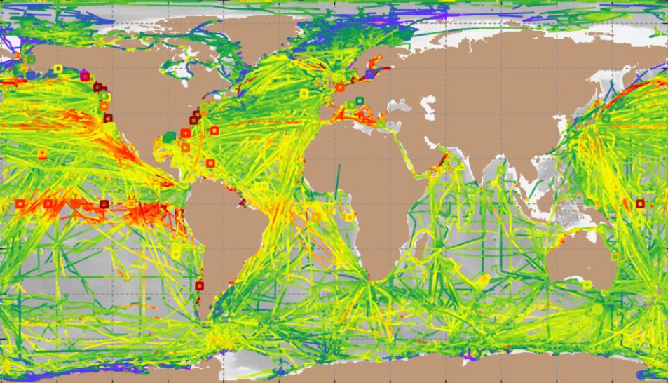
Map showing the surface ocean CO₂ from ships, drifters and autonomous surface platforms and moorings for all data in SOCAT version 2025, coloured by fCO2 concentration (scale not shown).

SOCAT v2025 is released today! A grand total of 49.6 million surface ocean fCO2 observations from dozens of contributors around the world.

www.socat.info/v2025

#ocean #co2

Fig. 4: Schematic of the primary processes impacting the flow of carbon through the Southern Ocean. The vertical section on the right depicts the two-dimensional carbon cycle that results from zonally and temporally averaging the four-dimensional variability.

Alison Gray provides an overview of the Southern Ocean carbon cycle

doi.org/10.1146/annu...

#SouthernOcean #carbon #co2

This official #UNOC3 side event is organised by @icos-ri.eu, #JPIOceans and @oceanfrontier.bsky.social, co-organised by @geomarkiel.bsky.social, #NORCE, @noc.ac.uk, @ifremer.bsky.social and IO-PAN. The event funded by @george-project.bsky.social. 🌊 Read more: www.icos-cp.eu/unoc3

From Science to Solutions: Advancing the Ocean Carbon System for Climate Action UN Ocean Decade Conference 2025 off-site side event hosted by ICOS, JPI Oceans & Ocean Frontier Institute .

Going to the UN Ocean Decade Conference 2025? Join the side event "From Science to Solutions: Advancing the Ocean Carbon System for Climate Action" to get the latest updates on efforts to improve the global carbon observation network.

Full details at www.icos-cp.eu/news-and-eve...

#OceanDecade

Tim DeVries and 34 co-authors(!) present the results of the RECCAP2 assessment of the Magnitude, Trends, and Variability of the Global Ocean Carbon Sink From 1985 to 2018.

doi.org/10.1029/2023...

#ocean #co2 #carbon