Tim Weiland

Gaussian Processes and Reproducing Kernels: Connections and Equivalences This monograph studies the relations between two approaches using positive definite kernels: probabilistic methods using Gaussian processes, and non-probabilistic methods using reproducing kernel Hilb...

We've written a monograph on Gaussian processes and reproducing kernel methods (with @philipphennig.bsky.social, @sejdino.bsky.social and Bharath Sriperumbudur).

arxiv.org/abs/2506.17366

Love the skeleton marketing

Tired of your open-source ML work not getting the academic recognition it deserves? 🤔 Submit to the first-ever CodeML workshop at #ICML2025! It focuses on new libraries, improvements to established ones, best practices, retrospectives, and more.
codeml-workshop.github.io/codeml2025/

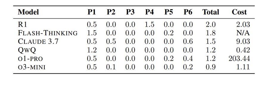
You’ve probably heard about how AI/LLMs can solve Math Olympiad problems ( deepmind.google/discover/blo... ).

So naturally, some people put it to the test — hours after the 2025 US Math Olympiad problems were released.

The result: They all sucked!

Excited to mention that this work was accepted to AISTATS 2025.
Shout-out to my amazing collaborators Marvin Pförtner & @philipphennig.bsky.social!

Flexible and Efficient Probabilistic PDE Solvers through Gaussian Markov Random Fields Mechanistic knowledge about the physical world is virtually always expressed via partial differential equations (PDEs). Recently, there has been a surge of interest in probabilistic PDE solvers -- Bay...

In summary: The SPDE perspective brings us more flexible prior dynamics and highly efficient inference mechanisms through sparsity.

📄 Curious to learn more? Our preprint: arxiv.org/abs/2503.08343
💻 And there's Julia code: github.com/timweiland/G... & github.com/timweiland/D...

8/8

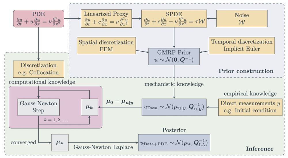
A diagram describing our method. You start with some PDE you want to solve. Then, you construct a linearized SPDE that closely resembles the dynamics of this PDE. Discretizing this SPDE (through FEM along space and some e.g. implicit Euler scheme along time) yields a GMRF prior with a sparse precision matrix. Then, you condition this prior on your (noisy) observations, e.g. the initial condition. Afterwards, you perform Gauss-Newton steps until convergence to integrate the (nonlinear) information about the PDE discretization. At convergence, you do Laplace to finally obtain a GMRF posterior over the solution of the PDE.

So here's the full pipeline in a nutshell:
Construct a linear stochastic proxy to the PDE you want to solve -> discretize to get a GMRF -> Gauss-Newton + sparse linear algebra to get a posterior which is informed about your data and the PDE. 7/8

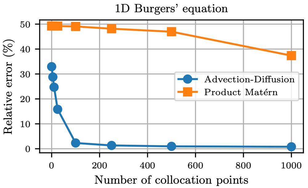
A plot comparing the two different priors we mentioned before for the task of solving a Burgers' equation. The x axis is the number of collocation points, and the y axis is the relative error in percentage. We observe that the advection-diffusion prior achieves a very low relative error already for a low number of collocation points, while the error drops off much more slowly for the Matérn-based prior.

Turns out that these "physics-informed priors" indeed then converge much faster (in terms of the discretization resolution) to the true solution. 6/8

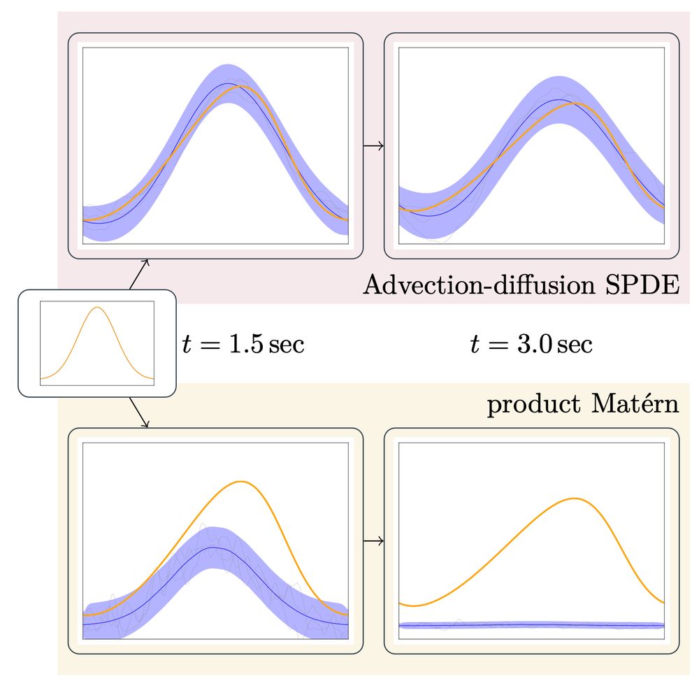
A diagram comparing the effect of different priors for probabilistic numerical PDE solvers. For the task of solving a Burgers' equation, we compare a product of 1D Matérns with a prior constructed from an advection-diffusion SPDE. Both priors are conditioned only on the initial condition, and then we plot for two different time points how the dynamics evolve. We see that for the Matérn-based prior, the effect of the observations simply "dies out" over time. By contrast, the advection-diffusion prior actually propagates the observations through time in a way that much more closely resembles the Burgers' equation dynamics we want to approximate.

But wait a sec...
With this approach, we express our prior belief through an SPDE.
Then why should we use the Whittle-Matérn SPDE?
Instead, why don't we construct a linear SPDE that more closely captures the dynamics we care about? 5/8

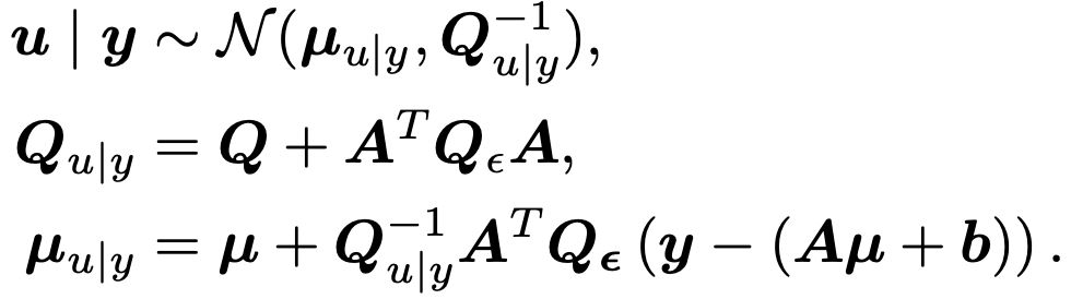
A screenshot of equations that express the posterior of a Gaussian Markov Random Field under affine observations y = Au + b.

Still with me?
So we get a FEM representation of the solution function, with stochastic weights given by a GMRF.
Now we just need to "inform" these weights about a discretization of the PDE we want to solve.
These computations are highly efficient, due to the magic of ✨sparse linear algebra✨. 4/8

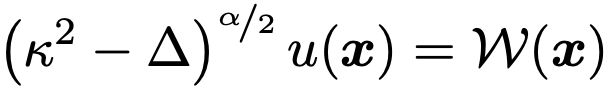
A screenshot of the equation for the Whittle-Matérn stochastic PDE.

Matérn GPs are solutions to the Whittle-Matérn stochastic PDE (SPDE).
In 2011, Lindgren et al. used the finite element method (FEM) to discretize this SPDE.
This results in a Gaussian Markov Random Field (GMRF), a Gaussian with a sparse precision matrix. 3/8

In the context of probabilistic numerics, people have been using Gaussian processes to model the solution of PDEs.
Numerically solving the PDE then becomes a task of Bayesian inference.
This works well, but the underlying computations involve expensive dense covariance matrices.
What can we do? 2/8

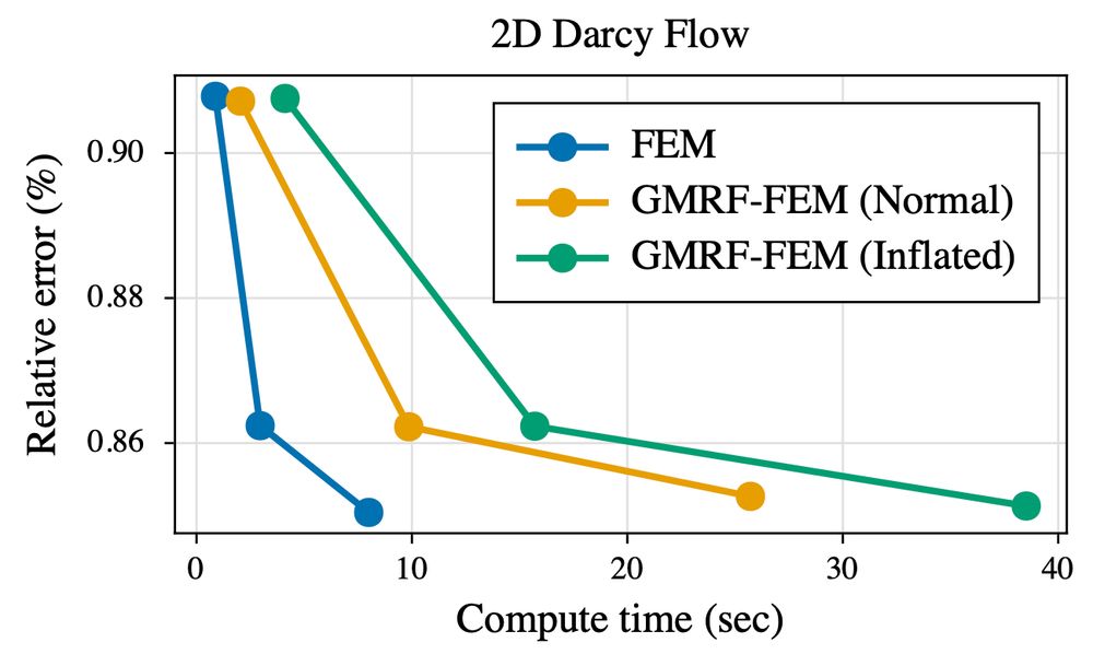
A plot comparing the performance of different methods to numerically solve PDEs. The x-axis depicts the compute time in seconds, the y-axis depicts the relative error to the ground-truth solution in percentage. The graph for the "standard" finite element method has the steepest downward slope and thus the best performance. Our methods based on Gaussian Markov Random Fields achieve the same accuracies as the finite element method, but at slight computational overheads, depicted by their graphs having a slightly flatter slope. For instance, the highest accuracy solves require ~8-9 seconds for FEM and ~25 seconds for our GMRF-based method.

⚙️ Want to simulate physics under uncertainty, at FEM accuracy, without much computational overhead?

Read on to learn about the exciting interplay of stochastic PDEs, Markov structures and sparse linear algebra that make it possible... 🧵 1/8

Reparameterization invariance in approximate Bayesian inference Current approximate posteriors in Bayesian neural networks (BNNs) exhibit a crucial limitation: they fail to maintain invariance under reparameterization, i.e. BNNs assign different posterior densitie...

Interestingly enough, these reparameterizations can indeed cause trouble in Bayesian deep learning. Check out arxiv.org/abs/2406.03334, which uses this same ReLU example as motivation :)

The submission site for ProbNum 2025 is now open! The deadline is March 5th. We welcome your beautiful work on probabilistic numerics and related areas!

probnum25.github.io/submissions

My recs: Doom emacs to get started; org mode + org-roam for notes, org-roam-bibtex + zotero auto-export for reference management; dired for file navigation; tramp mode for remote dev; gptel for LLMs; julia snail for julia, make sure you set up lsp. Start small and expand gradually, see what sticks

Amazing work! A big physics-informed ML dataset with actually relevant problems, created in cooperation with domain experts. It‘s time to finally move on from 1D Burgers‘ equations 🚀

I would also like to be added :) Great idea, thanks for this!

ELLIS PhD student here, I would also appreciate getting added :)